function KUPC_Radar_Simulation %Aug. 22, 2009
%{
1. This matlab program generates the radar simulation results of Figs. 4-7 reported in
the paper:
E.H. Feria, "On a Nascent Mathematical-Physical Latency-Information Theory, Part I:
The Revelation of Powerful and Fast Knowledge-Unaided Power-Centroid Radar",
Proceedings of SPIE Defense, Security and Sensing, Orlando Florida, April 2009.
Three observations regarding this April 2009 SPIE paper are:
a) It can be readily down-loaded from the author's Web-Site
'http://feria.csi.cuny.edu'.
b) It forms part of a USA as well as international patent application for the
radar techniques simulated by this MATLAB program as well as their natural
extensions to other types of applications.
c) Comments, suggestions, and/or queries regarding this MATLAB program and its
simulated algorithms can be sent to the author's E-Mail
'feria@mail.csi.cuny.edu'.
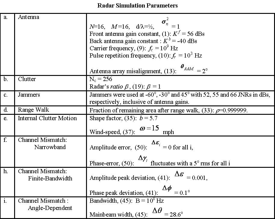
2. RADAR PARAMETER VALUES FOR THE SIMULATION RESULTS OF Figs. 4-7 of the above SPIE
paper are generated using the following parameter values specified in lines 26-72
(NOTE: Back clutter covariance is not simulated due to very small 'assumed' antenna
gain constant of Kb=-40dB specified in Table I of above SPIE paper.):
%}
N = 16; % Number of antenna elements
M = 16; % Number of CPI pulses
Nc = 256; % Number of range-bin cells
at = 0*pi/180; % Target angle of attack in radians
sn = 1; % Variance of antenna white noise
beta = 1; % Radar's ratio
aam = 2*pi/180; % Angle array misalignment
rho = .999999; % Range walk fraction
w = 15; % Internal clutter motion wind speed in miles/hr
b = 5.7; % Internal clutter motion shape factor
fr = 10^3; % Pulse repetition frequency in Hz
B = 10^8; % Angle dependent channel mismatch bandwidth in Hz
Kf = 56; % Front antenna gain constant in dBs
BeamWidth =28.6*pi/180; % Angle dependent channel mismatch mainbeam width
c = 2.9979*10^8; % Speed of light in meters per second
fc = 10^9; % Carrier frequency in Hz
De = 0.001; % Finite bandwidth channel mismatch amplitude peak dev.
Df = .1*pi/180; % Finite bandwidth channel mismatch phase peak dev.
DvRandom = 5*pi/180; % Narrowband channel mismatch phase peak deviation
dDL = 0.5; % Antenna inter-element distance to wavelength ratio
Ja(1) = -60*pi/180; % First jammer angle of attack of -60 degrees in radian
Jp(1) = 10^(34/10); % First jammer gain corresponding to 34 dBs
Ja(2) = -30*pi/180; % Second jammer angle of attack of -30 degrees in radian
Jp(2) = 10^(34/10); % Second jammer gain corresponding to 34 dBs
Ja(3) = 45*pi/180; % Third jammer angle of attack of 45 degrees in radian
Jp(3) = 10^(34/10); % Third jammer gain corresponding to 34 dBs
%{
The following four cases leading to Fig. 4-7 of above SPIE paper for 'Nj (the
number of jammers)' and 'Lev(the number of predicted clutter covariances)',
respectively, are next stated. More specifically, to generate Fig. 4 we let
Case = 4, for Fig. 5 we let Case = 5, for Fig. 6 we let Case = 6, and for Fig. 7
we let Case = 7;
%}
Case = 4;
if Case == 4 % Fig. 4
NJ = 3
Lev = 11
elseif Case == 5 % Fig. 5
NJ = 3
Lev = 3
elseif Case == 6 % Fig. 6
NJ = 0
Lev = 11
elseif Case == 7 % Fig. 7
NJ = 0
Lev = 3
end
%{<
3. NEXT THREE (3) GLOBAL CONTROL PARAMETERS ARE SPECIFIED FOR THE SIMULATION.
TWO (2) OF THE THREE PARAMETERS RESULT IN FASTER SIMULATIONS WHEN PREVIOUSLY EVALUATED
COVARIANCES ARE USED (specified with SAVED_Total_Covariance = 1) AND A PREVIOUSLY
EVALUATED SAMPLE COVARIANCE MATRIX INVERSE IS USED (specified with SAVED_SMI = 1).
Clearly, however, when the present MATLAB program is run for the first time it has
SAVED_Total_Covariance = 0 and SAVED_SMI = 0 to generate the required covariances that
are then stored for later use if the user wishes to do so.
THE THIRD AND LAST GLOBAL CONTROL PARAMETER SPECIFIES THE NUMBER OF PASSES OF THE SAR64
IMAGE THAT ARE USED TO OBTAIN THE SAMPLE COVARIANCE MATRIX INVERSE RESULTS FOR 64
RANGE-BINS. In particular, the number of these passes is specified by selecting a value
for Pass_SMI. Seven possible options for Pass_SMI are 1, 4, 8, 16, 20, 40 and 80.
FINAL TIMING NOTE: The running time, in author's laptop, to generate each figure of SPIE
paper flucturates from 10 to 20 minutes, depending on the case that is being simulated.
%}
SAVED_Total_Covariance = 0; % 0=NO and 1=Yes
SAVED_SMI = 0; % 0=NO and 1=Yes
Pass_SMI = 4; % Number of SAR image 'SAR64' iterations
% Possible options for Pass_SMI are 1,4,8,16,20,40 and 80
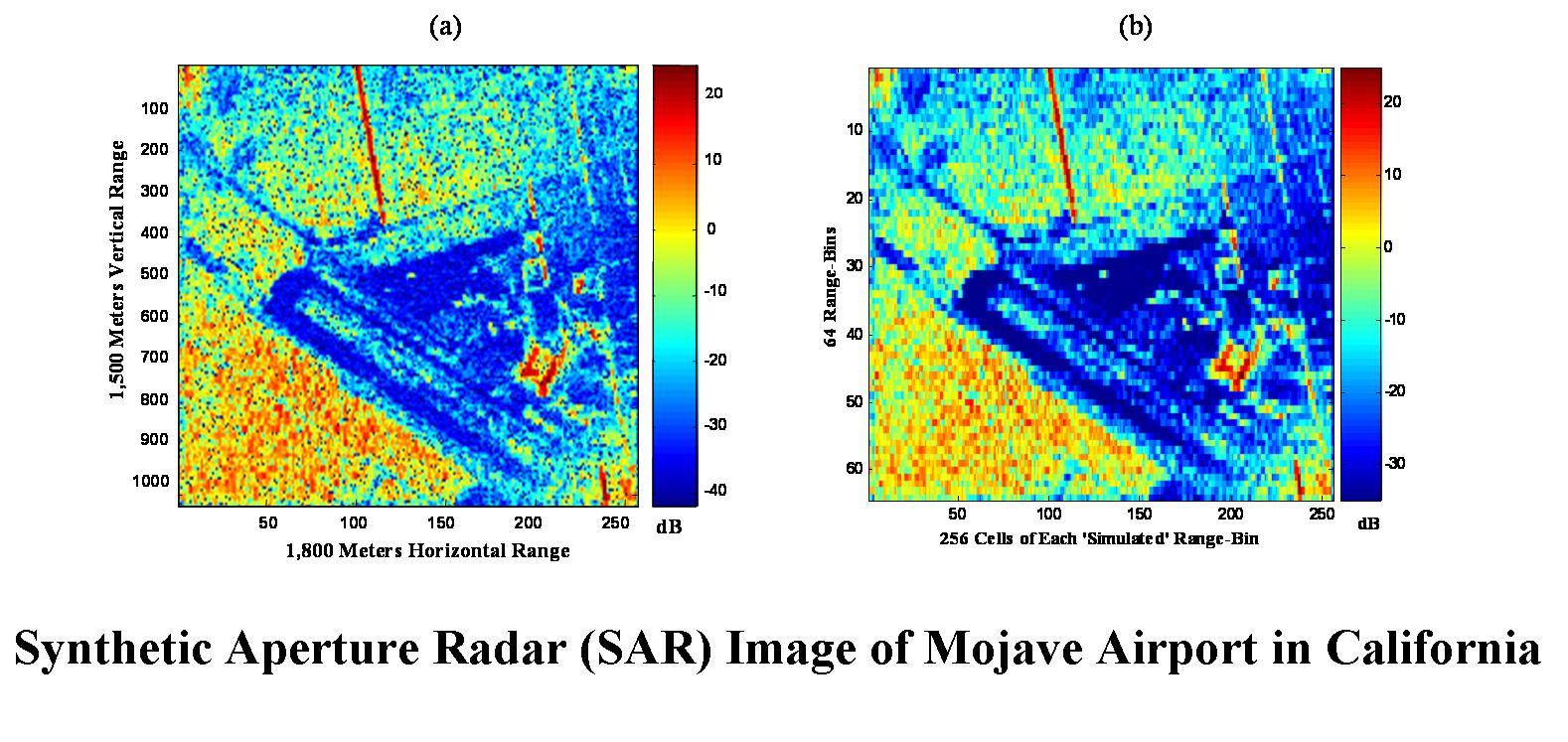
%%%% THIS PART OF PROGRAM FINDS POWER AND POWER-CENTROID OF 64 X 256 SAR IMAGERY LOADED
%%%% IN LINE 106 FOR BOTH BASELINE COMPARISONS AS WELL AS FOR SIMULATION OF THE SPIE
%%%% PAPER'S 'CLUTTER KNOWLEDGED-UNAIDED POWER-CENTROID RADAR' SCHEME
% The loading of the 1024 rows by 256 columns SAR image SAR1024
load ('sar_1024x256_2009','img2D_new_match');
SAR1024 = img2D_new_match;
% The generation of 64 rows (each row is an assumed range-bin) and 256 columns SAR
% image SAR64
for ii=1:64
SAR64(ii,:) = mean(SAR1024(16*ii-15:16*ii,:));
end
% The generation of 64 range-bins image times front antenna gain (see Eq.(1) in SPIE
% paper) SAR64g
HNc = Nc/2;
F((Nc+2)/2) = pi/(2*Nc);
for ii = 2: HNc
F(ii+ HNc) = F(ii+ HNc -1)+pi/Nc;
end
F(1: HNc) = -fliplr(F(HNc +1:2* HNc));
g = NormAntPat(N,Nc,dDL,F,at)*10^(Kf/10);
for ii=1:64
SAR64g(ii,:) = SAR64(ii,:).*g;
end
% 64 Power Evaluations from SAR64g
dBPower64 = 10*log10(sum(SAR64g'));
% 64 Power-Centroid Evaluations from SAR64g
Centro64 = Centroid(SAR64g);
%%%%% Next when one sets Option = 1 one displays the original SAR image
%%%%% 'SAR1024' as well as its 64 derived range-bins 'SAR64' together
%%%%% with its corresponding range-bin powers in dBs 'dBPower64' and
%%%%% range-bin power-centroids 'Centro64'
Option = 1;
if Option == 1
figure(11), imagesc([1 256], [1 1024], 10*log10(SAR1024), [-42 25]);
xlabel('256 Cells of Range-Bin Covering 1,800 Meters of Crossrange');
ylabel('64 SAR Range-Bins Covering 1,500 Meters of Downrange');
colorbar;
title('(a) SAR Resolution Cell Power in dBs for Original 1024x256 SAR');
figure(12), imagesc([1 256], [1 64], 10*log10(SAR64), [-35 25]);
xlabel('256 Cells of Range-Bin Covering 1,800 Meters of Crossrange');
ylabel('64 SAR Range-Bins Covering 1,500 Meters of Downrange');
colorbar;
title('(b) SAR Resolution Cell Power in dBs for 64 Range-Bins 64x256 SAR');
figure(13),plot(dBPower64),axis([1,64,30,85]);
xlabel('Range-Bin'); ylabel('Power in dBs');
title('(c) SAR-Antenna-Gain Power of 64 Range-Bins');
figure(14),plot(Centro64), axis([1,64,1,256]);
xlabel('Range-Bin'); ylabel('Centroid');
title('(d) SAR-Antenna-Gain Centroid of 64 Range-Bins');
end
tic
%%% THIS PART OF PROGRAM DERIVES TARGET STEERING VECTOR FOR L=101 NORMALIZED
%%% DOPPLER CASES AND Nc CLUTTER STEERING VECTORS
L = 101; % Odd-Number of Normalized Doppler Cases from -1/2 to 1/2
% Target Steering Vectors 'S' for L Normalized Doppler Cases (see Eqs. (4)-(7)
% of SPIE paper)
S = zeros(Nc,L);
VecN = 0:1:N-1;
VecM = 0:1:M-1;
FN = dDL*sin(at);
s1 = exp(i*2*pi*FN*VecN);
for kk = 1:L
FD = (kk-(L+1)/2)/(L-1);
ss1 = exp(i*2*pi*FD*VecM);
ss = transpose(kron(ss1,s1))/sqrt(N*M);
S(:,kk) = ss;
end
% Nc Clutter Steering Vectors 'V' ( see Eqs. (14)-(17) of SPIE paper)
V = zeros(N*M,Nc);
for ii = 1:Nc
FN = dDL*sin(F(ii));
c1 = exp(i*2*pi*FN*VecN);
FD = beta*dDL*sin(F(ii)+aam);
cc1 = exp(i*2*pi*FD*VecM);
cf = transpose(kron(cc1,c1));
V(:,ii) = cf;
end
%%% THIS PART OF PROGRAM FINDS JAMMER COVARIANCE 'CovJ'(see Eqs. (24)-(27) of SPIE paper)
CovJ = zeros(N*M,N*M);
for ii = 1:NJ
integ = round((Ja(ii)+pi/2)*Nc/pi);
FN = dDL*sin(F(integ));
c1 = exp(i*2*pi*FN*VecN);
cc1 = ones(1,M);
cf = transpose(kron(cc1,c1));
CovJ = CovJ+Jp(ii)*g(integ)*kron(eye(M),ones(N,N)).*(cf*cf');
end
%%%%%% THIS PART OF PROGRAM FINDS ASSUMED INTERFERENCE AND NOISE COVARIANCES
%%% White Noise Covariance 'Cwn' (see Eq. (22) of SPIE paper)
Cwn = sn*eye(N*M);
%%% Range Walk Covariance 'Crw' (see Eq. (30)-(32) of SPIE paper)
for ii=1:M
for jj=1:M
rwtime(ii,jj) = rho^abs(ii-jj);
end
end
Crw = kron(rwtime,ones(N,N));
%%% Internal Clutter Motion Covariance 'Cicm' (see Eqs. (34)-(36) of SPIE paper)
lda = c/fc;
Tr = 1/fr;
fcMHz = fc/10^6;
r = 10^((63.2-15.5*log10(w)-12.1*log10(fcMHz))/10);
for ii=1:M
for jj=1:M
icmtime(ii,jj) = (r+(b*lda)^2/((b*lda)^2+(4*pi*abs(ii-jj)*Tr)^2))/(r+1);
end
end
Cicm = kron(icmtime,ones(N,N));
%%% Finite Bandwidth Channel Mismatch Covariance 'cmfb' (see Eqs. (39)-(42) of SPIE paper)
for ii=1:N
for jj=1:N
if ii==jj
cmfbspace(ii,jj) = 1-De+De^2/3;
else
cmfbspace(ii,jj) = (1-De/2)^2*(sinc(Df/2))^2;
end
end
end
cmfb = kron(ones(M,M),cmfbspace);
%%% Angle Dependent Channel Mismatch Covariance 'cmad' (see Eqs. (43)-(46) of SPIE paper)
for ii=1:N
for jj=1:N
if ii==jj
cmadspace(ii,jj) = 1;
else
cmadspace(ii,jj) = sinc(B*sin(BeamWidth)*dDL/fc*abs(ii-jj));
end
end
end
cmad = kron(ones(M,M),cmadspace);
%%%%%%% In this part of program the total cvariance for all range bins 'Cov'
%%%%%%% (See Eq. (12) of SPIE paper with Cbc, the back clutter covariance, set to zero)
%%%%%%% is either evaluated or loaded. When the variable
%%%%%%% SAVED_Total_Covariance is equal to 1 Cov is loaded along
%%%%%%% with CovFc (the front clutter covariance of Eq. (13) of SPIE paper), Cov12
%%%%%%% (the squared root of the matrix Cov) and cmnb (the angle
%%%%%%% independent channel mismatch covariance).
%{
NOTE: When running this program for the first time it should always be run with
the variable SAVED_Total_Covariance set to 0 since all relevant covariances,
i.e. Cov, CovFc, Cov12, and cmnb must be evaluated and saved in the first run for
its later use if user wishes to do so
%}
if SAVED_Total_Covariance == 1
load Cov, load CovFc, load Cov12, load cmnb
else
% Angle Independent Channel Mismatch Covariance 'cmnb' is evaluated and saved here
DFVec = exp(i*randn(1,N)*DvRandom);
cmnb = [];
for ii=1:M
cmnb = [cmnb DFVec];
end
cmnb = transpose(cmnb)*conj(cmnb);
save cmnb cmnb;
% Cov, CovFc and Cov12 are evaluated and saved here
range_bins_SMI = [1:64];
for jj = range_bins_SMI
Ccf = zeros(Nc,Nc);
for ii = 1:Nc
cf = V(:,ii);
Ccf = Ccf+SAR64g(jj,ii)*cf*cf';
end
CovFc{jj} = Ccf;
Cov{jj} = Ccf.*((Crw.*Cicm).*((cmnb.*cmfb).*cmad))+CovJ.*((cmnb.*cmfb).*cmad)+Cwn;
Cov12{jj} = Cov{jj}^(1/2);
end
save Cov Cov, save CovFc CovFc, save Cov12 Cov12
end
%%% In this part of program the sample matrix inverse for one of a number of possible SAR
%%% image passes (1,4,8,16,20,40,80) yielding InvXC1,..,InvXC80,
%%% respectively is evaluated and saved (see Eqs. (53)-(55) of SPIE paper). This is also
%%% done with its associated moments m1,...,m80 (see Eqs. (74) and (75) for an example)
%%% which are used in the on-line evaluation of each range-bin power-centroids
%%% (See Eqs. (68), (69) and (76)). Also when the variable SAVED_SMI is
%%% equal to 1 InvXCi and mi is loaded when the variable Pass_SMI is
%%% equal to 'i'.
%{
NOTE: When running this program for the first time it should always be run with
the variable SAVED_SMI set to 0 since all the relevant information, i.e. InvXC'i' and
m'i', must first be evaluated and saved in the first run for its later use if user
wishes to do so
%}
if SAVED_SMI == 1
if Pass_SMI == 1
load InvXC1; load m1;
elseif Pass_SMI == 4
load InvXC4; load m4;
elseif Pass_SMI == 8
load InvXC8; load m8;
elseif Pass_SMI == 16
load InvXC16; load m16;
elseif Pass_SMI == 20
load InvXC20; load m20;
elseif Pass_SMI == 40
load InvXC40; load m40;
elseif Pass_SMI == 80
load InvXC80; load m80;
end
else
PCCME_Power_RB = zeros(N*M,N*M);
m = zeros(length(range_bins_SMI),N+M-1);
for jj = range_bins_SMI
%%%%%% SMI Statistics
PCCME_Power = zeros(N*M,N*M);
for ii = 1:Pass_SMI
XC = Cov12{jj}*randn(N*M,1);
PCCME_Power = PCCME_Power+XC*XC';
end
PCCME_Power_RB = PCCME_Power_RB+PCCME_Power;
%%%%%% Centroid Moments
Aux = PCCME_Power/Pass_SMI;
for ii = 1:N
m(jj,ii) = Aux(1,ii);
end
iter = N+1;
for ii = 2*N:N:M*N
m(jj,iter) = Aux(1,ii);
iter = iter+1;
end
end
PCCME_Power_RB = PCCME_Power_RB/(Pass_SMI*length(range_bins_SMI));
if Pass_SMI == 1
InvXC1 = inv(PCCME_Power_RB+10*eye(Nc)); cmnb1 = cmnb; m1 = m;
save InvXC1 InvXC1; save m1 m1
elseif Pass_SMI == 4
InvXC4 = inv(PCCME_Power_RB+10*eye(Nc)); cmnb4 = cmnb; m4 = m;
save InvXC4 InvXC4; save m4 m4
elseif Pass_SMI == 8
InvXC8 = inv(PCCME_Power_RB+10*eye(Nc)); cmnb8 = cmnb; m8 = m;
save InvXC8 InvXC8; save m8 m8
elseif Pass_SMI == 16
InvXC16 = inv(PCCME_Power_RB+10*eye(Nc)); cmnb16 = cmnb; m16 = m;
save InvXC16 InvXC16; save m16 m16
elseif Pass_SMI == 20
InvXC20 = inv(PCCME_Power_RB+10*eye(Nc)); cmnb20 = cmnb; m20 = m;
save InvXC20 InvXC20; save m20 m20
elseif Pass_SMI == 40
InvXC40 = inv(PCCME_Power_RB+10*eye(Nc)); cmnb40 = cmnb; m40 = m;
save InvXC40 InvXC40; save m40 m40
elseif Pass_SMI == 80
InvXC80 = inv(PCCME_Power_RB+10*eye(Nc)); cmnb80 = cmnb; m80 = m;
save InvXC80 InvXC80; save m80 m80
end
Pass_SMI
end
if Pass_SMI == 1
InvXC = InvXC1; MM = m1;
elseif Pass_SMI == 4
InvXC = InvXC4; MM = m4;
elseif Pass_SMI == 8
InvXC = InvXC8; MM = m8;
elseif Pass_SMI == 16
InvXC = InvXC16; MM = m16;
elseif Pass_SMI == 20
InvXC = InvXC20; MM = m20;
elseif Pass_SMI == 40
InvXC = InvXC40; MM = m40;
elseif Pass_SMI == 80
InvXC = InvXC80; MM = m80;
end
%%%% In this part actual and on-line estimated power-centroids and power
%%%% for all 64 Range-bins are derived
% Antenna directions for use in yielding quantized power-centroid values
% according to specified quantization levels 'Lev'
Dev = Nc-1;
Dir_Boundary = [Dev/Lev:Dev/Lev:Dev-Dev/Lev]+1;
Antenna_Dir = [Dir_Boundary Dev+1]-0.5*Dev/Lev;
for jj = 1:64
% Next quantized power-centroids 'PCCQ_Cent' are evaluated making use of Eqs. (68),
% (69) and (76) with kcen=60 of SPIE paper. Unquantized centroids 'PCCM_Centroids'
% and 'PCCME_Centroids' are also found from the moments derived from 'MM' and 'CC',
% respectively.
kcen = 60;
CC = Cov{jj};
% Here Power and Power-Centroids are Evaluated From Moments of the
% True Clutter Covariance Cov
for ii = 1:N
mc(ii) = CC(1,ii);
end
iter = N+1;
for ii = 2*N:N:M*N
mc(iter) = CC(1,ii);
iter = iter+1;
end
mmntc = 0;
Lengt = length(mc)-1;
for ii = 2:1+Lengt
mmntc = mmntc + mc(ii)*(-1)^ii*2^(Nc-ii)/2^(Nc-2);
end
PCCM_Centroids(jj) = (Nc+1)/2-kcen*imag(mmntc)/mc(1);
dBPowerClu(jj) = 10*log10(real(mc(1)));
% Here Power and Power-Centroids are Evaluated From Moments Derived
% From On-Line Sample Covariance Matrix MM
m = MM(jj,:);
mmnt = 0;
for ii = 2:1+Lengt
mmnt = mmnt + m(ii)*(-1)^ii*2^(Nc-ii)/2^(Nc-2);
end
PCCME_Centroid(jj) = (Nc+1)/2-kcen*imag(mmnt)/m(1);
dBPowerCluEst(jj) = 10*log10(real(m(1)));
% Here Quantized Power-Centroids are Evaluated From Unquantized Power-Centroids
% Evalued From Moments of On-Line Sample Covariance Matrix MM
PCCQ_Cent(jj) = Antenna_Dir(Lev);
for ii = 1:Lev-1
if PCCME_Centroid(jj) < Dir_Boundary(ii)
PCCQ_Cent(jj) = Antenna_Dir(ii);
break
end
end
end
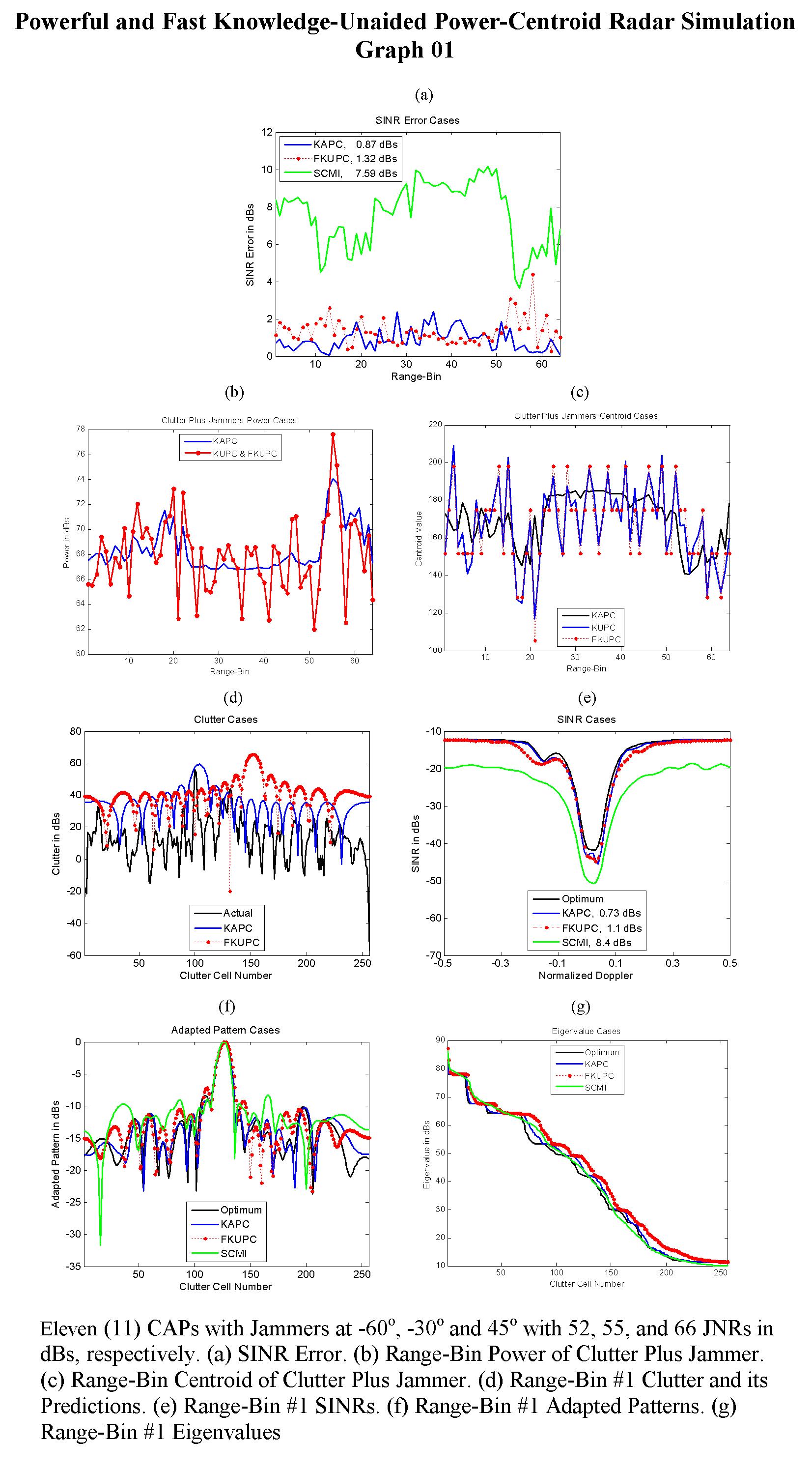
%{
In this part of program graphs with (when NJ>0) or without (when NJ=0) jammer are
produced for three 'clutter power' and 'clutter power-centroid' cases. These three
cases are:
1. KAPC: Knowledge Aided Power-Centroid (KAPC) Radar Case of Eqs. (57)-(58).
2. KUPC: Knowledge Unaided Power-Centroid (KUPC) Radar Case of Eqs. (65)-(66).
3. FKUPC: Fast Knowledge Unaided Power-Centroid (FKUPC) Radar Case of Eqs. (92)-(93).
%}
if NJ > 0
x = [1:64];
y1 = PCCM_Centroids; y2 = PCCME_Centroid; y3 = PCCQ_Cent;
figure(2), plot(x,y1,'-k',x,y2,'--b',x,y3,'-.r','LineWidth',2);
y = [120:160];
legend('KAPC','KUPC','FKUPC',3,'Location','SouthWest');
xlabel('Range-Bin');
ylabel('Centroid Value');
title('(b) Clutter Plus Jammers Centroid Cases');
y2 = dBPowerClu; y3 = dBPowerCluEst;
figure(3), plot(x,y2,'--b',x,y3,'-.r','LineWidth',2);
legend('KAPC','KUPC & FKUPC',2,'Location','North');
xlabel('Range-Bin');
ylabel('Power in dBs');
title('(c) Clutter Plus Jammers Power Cases');
else
x = [1:64];
y1 = Centro64; y2 = PCCME_Centroid; y3 = PCCQ_Cent;
figure(2), plot(x,y1,'-k',x,y2,'--b',x,y3,'-.r','LineWidth',2);
legend('KAPC','KUPC','FKUPC',3,'Location','South');
xlabel('Range-Bin');
ylabel('Centroid Value');
title('(b) Clutter Centroid Cases');
y1 = dBPower64; y2 = dBPowerCluEst; y3 = dBPowerCluEst;
figure(3), plot(x,y1,'-k',x,y2,'--b',x,y3,'-.r','LineWidth',2);
legend('KAPC','KUPC & FKUPC',3,'Location','North');
xlabel('Range-Bin');
ylabel('Power in dBs');
title('(c) Clutter Power Cases');
end
%{
In this part of program the SINR in dBs of four different algorithms are evaluated for
the considered range-bins. These algorithms are:
1. dBSINROpt: Optimum SINR of Eq. (52)
2. dBSINRPCCT: Suboptimum SINR of KAPC derived from Eq. (3) with w expression given
by Eq. (57)
3. dBSINRPCCQ: Suboptimum SINR of FKUPC derived from Eq. (3) with w expression given
by Eq. (92)
4. dBSINRSMI: Suboptimum SINR of SCMI derived from Eq. (3) with w expression given
by Eq. (53)
In addition, to the SINR results, the remaining results presented in Figs. 4-7
are also generated here.
%}
range_bins = [1:64]; % The Processed Range Bins
Clu_Opt = zeros(length(range_bins),Nc);
Clu_PCCT = zeros(length(range_bins),Nc);
Clu_PCCQ = zeros(length(range_bins),Nc);
Eig_Opt = zeros(length(range_bins),Nc);
Eig_PCCT = zeros(length(range_bins),Nc);
Eig_PCCQ = zeros(length(range_bins),Nc);
Eig_SMI = zeros(length(range_bins),Nc);
for jj = range_bins
Ccf = CovFc{jj};
C = Cov{jj};
m = MM(jj,:);
Power_True = dBPower64(jj);
Power_Mom = dBPowerClu(jj);
Power_Mom_Est = dBPowerCluEst(jj);
Cntrd_True(jj) = Centro64(jj);
Cntrd_Q(jj) = PCCQ_Cent(jj);
%%%% Derivation of predicted clutter covariance (PCC) 'PCC_true', Eq. (59),
%%%% is done using true centroids 'Centro64' of SAR image (see Eqs. (60)-(63))
%%%% as was done earlier when finding Centro64 (see line 95).
gT = NormAntPat(N,Nc,dDL,F,(Centro64(jj)-(Nc+1)/2)*pi/Nc);
PCC = zeros(Nc,Nc);
for ii = 1:Nc
cf = V(:,ii);
PCC = PCC+gT(ii)*cf*cf';
end
PCC_true = PCC/PCC(1,1)*Ccf(1,1);
%%%% Derivation of PCC 'PCCQ', Eq. (67), using 'quantized' centroids
%%%% 'PCCQ_Cent' ( see line 375 )
gQ = NormAntPat(N,Nc,dDL,F,(PCCQ_Cent(jj)-(Nc+1)/2)*pi/Nc);
PCC = zeros(Nc,Nc);
for ii = 1:Nc
cf = V(:,ii);
PCC = PCC+gQ(ii)*cf*cf';
end
PCCQ = PCC/PCC(1,1)*m(1);
% Three Clutter Cases
dBCluOpt(jj,:) = 10*log10(SAR64g(jj,:));
dBCluPCCT(jj,:) = 10*log10(Ccf(1,1)*gT);
dBCluPCCQ(jj,:) = 10*log10(m(1)*gQ);
% Four Eigenvalue Cases
Cdis = (Crw.*Cicm).*((cmnb.*cmfb).*cmad);
CJn = CovJ.*((cmnb.*cmfb).*cmad)+Cwn;
CPCCT = PCC_true.*Cdis+CJn;
CPCCQ = PCCQ.*Cdis+CJn;
dBEigOpt(jj,:) = 10*log10(flipud(sort(abs(eig(C)))));
dBEigPCCT(jj,:) = 10*log10(flipud(sort(abs(eig(CPCCT)))));
dBEigPCCQ(jj,:) = 10*log10(flipud(sort(abs(eig(CPCCQ)))));
dBEigSMI(jj,:) = 10*log10(flipud(sort(abs(eig(inv(InvXC))))));
% Four Adapted Pattern Cases
Cinv_Opt = inv(C);
Cinv_True = inv(CPCCT);
Cinv_Q = inv(CPCCQ);
for hh = 1:Nc
APOpt(jj,hh) = abs(S(:,(L+1)/2)'*Cinv_Opt'*V(:,hh));
APPCCT(jj,hh) = abs(S(:,(L+1)/2)'*Cinv_True'*V(:,hh));
APPCCQ(jj,hh) = abs(S(:,(L+1)/2)'*Cinv_Q'*V(:,hh));
APSMI(jj,hh) = abs(S(:,(L+1)/2)'*InvXC'*V(:,hh));
end
dBAPOpt(jj,:) = 10*log10(APOpt(jj,:)/max(APOpt(jj,:)));
dBAPPCCT(jj,:) = 10*log10(APPCCT(jj,:)/max(APPCCT(jj,:)));
dBAPPCCQ(jj,:) = 10*log10(APPCCQ(jj,:)/max(APPCCQ(jj,:)));
dBAPSMI(jj,:) = 10*log10(APSMI(jj,:)/max(APSMI(jj,:)));
% Four SINR Cases
for kk = 1:L
s = S(:,kk);
w1 = Cinv_Opt*s; dBSINROpt(jj,kk) = 10*log10(real(w1'*s*s'*w1)/real(w1'*C*w1));
w2 = Cinv_True*s;dBSINRPCCT(jj,kk) = 10*log10(real(w2'*s*s'*w2)/real(w2'*C*w2));
w5 = Cinv_Q*s; dBSINRPCCQ(jj,kk) = 10*log10(real(w5'*s*s'*w5)/real(w5'*C*w5));
w6 = InvXC*s; dBSINRSMI(jj,kk) = 10*log10(real(w6'*s*s'*w6)/real(w6'*C*w6));
end
end
%%%%%% Range-Bin #1 Displayed Images of Figs. 4-7
range_bins = [1];
for jj = range_bins
v0 = dBCluOpt(jj,:); v1 = dBCluPCCT(jj,:); v4 = dBCluPCCQ(jj,:);
x = [1:256];
figure(4), plot(x,v0,'-k',x,v1,'--b',x,v4,'-.r','LineWidth',2);
xlim([1,256])
legend('Actual','KAPC','FKUPC',3,'Location','South');
xlabel('Clutter Cell Number');
ylabel('Clutter in dBs');
title('(d) Clutter Cases');
v0 = dBSINROpt(jj,:); v1 = dBSINRPCCT(jj,:); v4 = dBSINRPCCQ(jj,:);
v5 = dBSINRSMI(jj,:);
x = [-0.5:.01:0.5];, y = [0:5:65];
figure(5), plot(x,v0,'-k',x,v1,'--b',x,v4,'-.r',x,v5,':g','LineWidth',2);
legend('Optimum','KAPC, XXX dBs','FKUPC, XXX dBs','SCMI, XXX dBs',4,'Location','South');
xlabel('Normalized Doppler');
ylabel('SINR in dBs');
title('(e) SINR Cases');
v0 = dBAPOpt(jj,:); v1 = dBAPPCCT(jj,:); v4 = dBAPPCCQ(jj,:);
v5 = dBAPSMI(jj,:);
x = [1:256];
figure(6), plot(x,v0,'-k',x,v1,'--b',x,v4,'-.r',x,v5,':g','LineWidth',2);
xlim([1,256])
legend('Optimum','KAPC','FKUPC','SCMI',4,'Location','South');
xlabel('Clutter Cell Number'); ylabel('Adapted Pattern in dBs');
title('(f) Adapted Pattern Cases');
v0 = dBEigOpt(jj,:); v1 = dBEigPCCT(jj,:); v4 = dBEigPCCQ(jj,:);
v5 = dBEigSMI(jj,:);
x = [1:256]; y = [0:10:100];
figure(7), plot(x,v0,'-k',x,v1,'--b',x,v4,'-.r',x,v5,':g','LineWidth',2);
xlim([1,256])
legend('Optimum','KAPC','FKUPC','SCMI',4,'Location','North');
xlabel('Clutter Cell Number');
ylabel('Eigenvalue in dBs');
title('(g) Eigenvalue Cases');
DB_error_KAPC = mean(dBSINROpt(jj,:)-dBSINRPCCT(jj,:))
DB_error_FKUPC = mean(dBSINROpt(jj,:)-dBSINRPCCQ(jj,:))
DB_error_SCMI = mean(dBSINROpt(jj,:)-dBSINRSMI(jj,:))
end
range_bins = [1:64];
for jj = range_bins
ASMEdB_PCCT(jj) = mean(dBSINROpt(jj,:)-dBSINRPCCT(jj,:));
ASMEdB_PCCQ(jj) = mean(dBSINROpt(jj,:)-dBSINRPCCQ(jj,:));
ASMEdB_SMI(jj) = mean(dBSINROpt(jj,:)-dBSINRSMI(jj,:));
end
Avg_DB_error_KAPC = mean(ASMEdB_PCCT)
Avg_DB_error_FKUPC = mean(ASMEdB_PCCQ)
Avg_DB_error_SCMI = mean(ASMEdB_SMI)
w1 = ASMEdB_PCCT; w4 = ASMEdB_PCCQ;
w5 = ASMEdB_SMI;
x = [1:64];
figure(1), plot(x,w1,'--b',x,w4,'-.r',x,w5,':g','LineWidth',2);
Legend('KAPC, XXX dBs','FKUPC, XXX dBs','SCMI, XXX dBs',3,'Location','NorthWest');
xlabel('Range-Bin'); ylabel('SINR Error in dBs');
title('(a) SINR Error Cases');
toc
end
function g = NormAntPat(N,NC,dDL,F,at)
for ii = 1:NC
g(ii) = (sin(N*pi*dDL*(sin(F(ii))-sin(at)))/sin(pi*dDL*(sin(F(ii))-sin(at))))^2;
end
g=g/N^2;
end
function C=Centroid(SARg);
[RBN,NC]=size(SARg);
for ii = 1:RBN
C(ii) = 0;
for jj =1:NC
C(ii) = C(ii)+jj*SARg(ii,jj);
end
C(ii)=C(ii)/sum(SARg(ii,:));
end
end
function C=CentroidNew(SARg,int);
[RBN,NC]=size(SARg);
for ii = 1:RBN
C(ii) = 0;
for jj =1:NC
C(ii) = C(ii)+int(jj)*SARg(ii,jj);
end
C(ii)=C(ii)/sum(SARg(ii,:));
end
end
function SNR = Signal_to_Noise_Ratio(Image, ImageN)
[x,y]=size(Image);
powerr= 0;
error = 0;
for ii=1:x
for jj=1:y
powerr = powerr+Image(ii,jj)^2;
error = error+(Image(ii,jj)-ImageN(ii,jj))^2;
end
end
SNR = 10*log10(powerr/error);
end